The Numerical Integration Problem

A famous mathematical problem that is easy to compute is to approximate the numerical value of a definite integral of a function from a to b as the area under the curve of that function using the rectangle method.

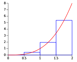
Given a function, we can approximate its definite integral over the interval (a, b) by adding the values of the areas of contiguous small rectangles whose heights are the value of the function along the interval. Zoomed in on a small portion of a curve for a function, these rectangles look like this:

This image is courtesy of Qref on Wikimedia commons.

Programming Numerical Integration

Programs written for solving this problem on a given function are fairly straightforward and involve determining the number of rectangles desired over a given interval and computing the value of the function for each rectangle, adding it to an overall sum for the value of the integral.

For a sequential implementation of such a program, the run time is on the order of the number of rectangles. To obtain an accurate result, a large number of rectangles should be used.

The sample code we provide in area.tgz contains a program that will enable you to visualize several ways that we can make numerical integration run faster by splitting the work of computing the area of each of the rectangles across multiple processing units. In these examples, we illustrate the types of data decomposition patterns that can be used. In this problem, the data to be computed is the area of each rectangle and we can think of those rectangles as lining up linearly along the x axis as shown above. In the following sections we will walk you through the execution of this code for several different data decompositions of this linear collection of rectangles, using a simple function.

The code you will use is not necessarily meant for you to examine, but instead to run with different hardware and software combinations and see how the decomposition took place. We built the code to execute in real time, saving the results of which processing unit computed which rectangle. We then graphically display the results by replaying the computations, drawing the rectangles with a time delay so you can visualize what happened.

Continue to the next chapter to begin your journey!